In the first four weeks of deep learning, I was under the impression that any learning problem could be solved by a big enough MLP with thorough enough tuning, that architecture didn't matter so much. I even asserted that manual tuning got me better results than using a scheduler to adjust learning rate.

Well, six weeks in, HW2 Kaggle competition is done, and I'm back with a few amendments:

• Yes, architecture does matter to an extent.
• I did NOT rely on tuning, not to the butt-glued-to-my-chair extent that I did for HW1 Kaggle. No more manually tuning learning rate, the scheduler is good enough, I can leave my chair!

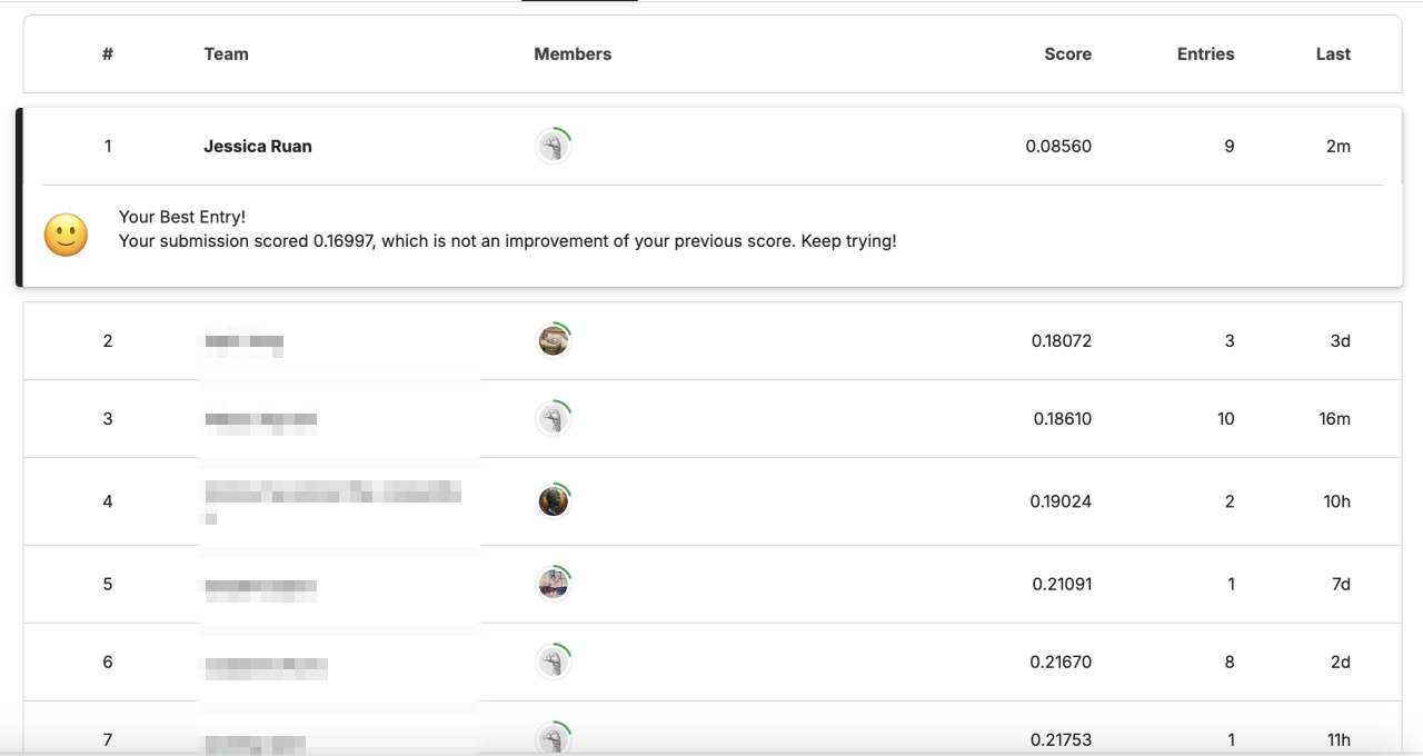
If HW1P2 was "tuning is king," HW2P2 is "data is king." I stumbled upon one weird trick that was unreasonably effective and stuck with it for the rest of the competition.

The moment I stumbled upon my "one weird trick"! I actually finished in 11th place, but I think the leap to EER < 0.10 has the most interesting discussion.

Facial Recognition

These days, when I see a new face, it often rhymes with a face I've seen before. Like, "They could pass as an aunt of this other person I know," or, "Looks like a sum of these two faces, minus this other face."

At 21 years old, I've seen enough faces for this rhyming phenomenon to happen. Apparently I can expect to see 5,000 to 10,000 unique faces in my lifetime. The search results I get for "how many faces do people see in a lifetime" vary, but you get the point, it's a lot of faces!

A neural network can look at far more faces than I do. How do neural networks recognize faces?

The Measure: Classification is Not Verification

Classification asks, Given this photo, who's this person? Each unique person that the photo can be of is a class.

Verification asks, Given two photos, are they the same person, yes or no? To be more precise, we're given a single photo and asked, "Given this photo, is it a photo of someone I know, or is it none of the above?" But it reduces to walking through our roster of known people and asking, "Does our photo match this person we're looking at, yes or no?"

Classification and verification are not the same! In particular, being good at classification doesn't mean we'll be good at verification, and vice versa.

To understand why, let's first define how we're measuring "good at classification" and "good at verification." We're good at classification if we have a high percentage of correctly classified images out of all images we classified. As for verification, we're good at verification if we have a low equal error rate (EER) score; that is, EER is the threshold at which the false positives rate equals the false negatives rate, and we want this threshold to be low.

Now, why does having a high classification accuracy (good at classification) not bestow a low EER score (good at verification)?

To classify a photo, to say this photo is Class X and not any other class, you need it to score higher for Class X than any other class, by being closest to the feature vector your model learned for Class X.

To verify a pair of photos, to say yes, these photos are of the same person, you need their pairwise similarity score to be higher than the threshold used to calculate EER. This is independent of classification.

Now, in HW2, our task was to tackle verification and get our EER as low as possible. To tackle verification, we must train our models for classification, but the one thing to note is that we're not optimizing for classification, but for verification.

This distinction will be important when taking the one weird trick into account.

The Architecture: MLP vs CNNs

First, let's put the facial recognition problem aside, and answer an easier question: Given a photo, does it have a face in it?

In theory, if we have a big enough MLP, it'll be able to solve the facial recognition task.

So why don't we use one big MLP?

Suppose we answer this question with one big MLP. We flatten the photo into a 1D vector and feed it into the MLP.

One component of this MLP answers the question, Does this segment in the top-left corner of the photo have a face in it? Another component of this MLP answers the question, Does this segment, slightly shifted right from the top-left corner of the photo have a face in it?, and so on.

Further suppose that the image is 1024x1024 pixels, and the face is small, like 50x50 pixels. (These numbers are hypothetical to illustrate how expensive MLPs can get; the images in our actual problem are 112x112 pixels.)

Well, this MLP will be huge, it'll take forever to train, and your computer can bake a potato.

Convolutional Neural Networks

Recall that the big MLP essentially has a component for each 50x50 segment of the photo, to ask Does this segment in the top-left corner of the photo have a face in it? and Does this segment, slightly shifted right from the top-left corner of the photo have a face in it?

Why not have a single small MLP, that takes a 50x50 segment and asks, Does this segment have a face in it? We scan this small MLP across the entire input, so we're essentially learning the parameters for this MLP rather than the one big MLP.

We call the weights matrix of this small MLP the convolution filter or kernel, and we say that we convolve this kernel with the input. 3Blue1Brown's But What is a Convolution? best visualizes the convolution process.

Aside from reducing the amount of parameters, CNNs are great at capturing intuitive invariances of images. Can watch this for a big picture overview, and the lecture slides and readings here if you want to dig more in depth.

Training Strategy: Data is King

I relied on two main techniques:

• Data augmentation. This was what brought my EER down from ~0.27 to ~0.18.
• One weird trick. This was what brought my EER down from ~0.18 to 0.08560, then polished down to 0.04714.

Data Augmentation

Perhaps the following exchange best illustrates the idea of data augmentation. I won't say which cousin, only that it happened when they were really young:

"What's this word?"

"Mickey Mouse!"

"Nice work!" I erase the Mickey, leaving only Mouse.

"Okay, what's this word?" Crickets.

I struggled with overfitting in the first few days. My model would have phenomenal classification accuracy, a whopping 99.8869% for training and 90.3208% for validation.

But! Classification is not verification!

While validation classification accuracy shot up into the 90+%, validation retrieval accuracy stalled at 73%, a sign of overfitting. My model stared at the faces for the retrieval task with the same astonishment that the three-year-old had with "Mouse."

Like how erasing the "Mickey" in "Mickey Mouse" gives us a totally new example, "Mouse," for our three-year-old to learn, we can transform our images to give our model totally new examples to learn. Eventually, our model will fight off overfitting and recognize "Mouse," or in our case learn to distinguish faces for the retrieval task instead of merely memorizing faces for classification.

For each training epoch, I apply two transformations to each image. The first transformation is a geometric-related one from Set 1 {no-op, flip, rotate, affine, random crop boundary, random crop rectangle from middle}, while the second transformation is a color-related one from Set 2 {no-op, color jitter, auto augment}.

I found that separating my transformations into two sets significantly reduced overfitting, as it increased the combinations of transformations to (5 + 1) x (2 + 1) = 18 transformations. Previously, I put Set 1 and Set 2 together into one set, making for only 5 + 2 + 1 = 8 transformations.

This data augmentation strategy gave me 431k images * 18 transformations = 7.7 million training images. I could play with more transformations, but my model enjoyed enough improvement that I left my data augmentation strategy like this.

One Weird Trick

Okay, now for the one weird trick! I think this was unreasonably effective given how simple it was and would love thoughts on why it's so effective.

I got the idea from the FixRes Mitigation section in this PyTorch blog post.

It's easy to miss because the Pytorch post makes FixRes sound incremental ("the above optimization improved our [classification] accuracy by an additional 0.160 points"), whereas it more than halved my EER score for the verification task.

To be fair, classification accuracy and verification EER are different measures. (Source)

The authors mentioned that they got an accuracy boost by training Resnet with a lower resolution than that of validation; in other words, their test and validation datasets were 224x224 pixel images, but they trained their model on 160x160 pixel images.

Since my images were 112x112 pixels, I wondered what would happen if I trained my model on 112x112 images, then validated them on 224x224 images.

To my surprise, after resizing my validation datasets, my validation EER for the verification task got a huge boost. This was the run when I discovered the unreasonable effectiveness of FixRes, and this was my best verification model if we control model size. The models I trained afterwards, that achieved better verification scores, were accomplished by scaling up model size, but their core idea remains the same.

Strangely, this FixRes trick only applies to verification, not classification. When I resized images to 224x224 for classification validation, I saw the opposite effect, a huge drop in classification accuracy. Hence, I preserved the 112x112 image sizes for classification validation.

Why this trick works: I theorize that this trick is kind of like dropout, in that it forces the network to extract less information. When you convolve a kernel with a small image, the kernel will squish a much wider area than it would if you convolve it with an enlarged version of the same image. So, when we train the network on 112x112 images and later validate it using larger images 224x224, it has an easier time with validation.

It's similar to athletes training at higher altitudes with less oxygen, then being dropped into the race at a normal altitude with normal oxygen levels.

Open question: The FixRes trick is great for verification, terrible for classification. When I resized images to 224x224 for classification validation, I saw the opposite effect, in that classification accuracy suffered. Why?

Ending

I think this one weird trick, the resolution trick that brings us the leap to EER < 0.10, has the most interesting discussion.

Once we make the leap into the EER < 0.10 club, the cockfight that goes on within the club is rather anticlimatic. Who has the biggest model wins, basically. (Unlike HW1, HW2 removed an upper restriction for number of parameters.) Humming along the wheels of capitalism, I scaled up my model and got EER down to 0.04714.

I stopped when my ratio of time spent butt-glued-to-chair outweighed the time spent saying "Wow!" Though, I think I took away enough "Wow" moments for the time to be worth it. The changes to my prior beliefs are:

• yes, big model train long = success, BUT
• architecture matters if you want to reduce parameters and thus training time. CNNs are cool!
• don't tune manually, it's not a hammer to your nails
• good classification accuracy != good verification accuracy, and in general we should have multiple measures when evaluating something
• data is king, some neat tricks you can do with data for unreasonably good results
• the FixRes trick is probably the first time my results matched (and exceeded) my expectations. It's exciting when you read about something and try it, and oh my word, it works