Inference Engines 1/N: KV Cache
I recommend you start from the beginning, from part 0/N.
- Inference Engines 0/N: Foundations
- Inference Engines 1/N: KV Cache <- we are here
- Inference Engines 2/N: Batching and PagedAttention
- Inference Engines 3/N: Speculative Decoding
Experiments: Original research that build on the Inference Engine series. Each piece will link back to
- Mixture of Experts. Or, When SpecDec Meets A Committee
Review of Phase 0
We're picking up where we left off. Remember our white whale?
out = lm.model(input_ids=input_ids, use_cache=False)
And remember the benchmarking harness we built around it? Here were our Phase 0 numbers:
model=gpt2 runs=3
  tokens/sec:    180.50
  ms/token:      5.54  (steady-state, decode)
  TTFT:          5.4 ms    (prefill)
  peak memory:   267 MB
Before we touch a single line of code, let's make sure we understand what these numbers mean and what we should expect to happen to them in an ideal world. If you can answer these questions, you understood Phase 0. If you can't, go reread it; take your time, I'll wait. :]
Question 1: What does TTFT measure, and why is it reported separately from ms/token?
Question 2: In Phase 0, TTFT and ms/token are nearly identical (~5.4 vs ~5.54 ms). Why? Would you expect them to stay nearly identical if we generated, say, 1024 tokens instead of 64?
Question 3: Now, suppose we find a way to avoid rereading the entire memo on every iteration. The LLM reads the prompt once, and from then on, it only looks at one new token per step. As we generate longer and longer sequences, which of our four metrics would you expect to behave differently than they did in the no-cache sweep, and how?
Phase 1, Step 1: Flipping the Magical use_cache from False to True
Commit: e966461
You raise your hand.
"The title of the post is KV Cache," you say.
"That is true," I say.
"And in our white whale, there's a... use_cache parameter," you say.
"That is also true," I say. "Very astute of you! What do you say we do with this... use_cache?"
Say it with me, boys and girls. Roses are red, violets are blue,
We flip this special use_cache parameter from False...
out = lm.model(input_ids=next_id, use_cache=False)
...to True.
out = lm.model(input_ids=next_id, use_cache=True)
Then we run our benchmarks...
modal run ./modal_run.py::main --check
...and our numbers shoot to the moon!
model=gpt2 runs=3
  tokens/sec:    999,999.99 🤑🤑
  ms/token:      0ms  (steady-state, decode)
  TTFT:          5.4 ms    (prefill)
  peak memory:   267 MB
That's KV Cache, boys and girls! We're all winners! See you next week!
Directed by Jessica Ruan
Written by Jessica Ruan
Produced by Jessica Ruan
Executive Producers Jessica Ruan Jessica Ruan Jessica Ruan
Co-Producer Jessica Ruan
Associate Producer Jessica Ruan
Not so fast. Here are the actual numbers, which are, er, not too different from Phase 0.
model=gpt2 runs=3
  tokens/sec:    162.52
  ms/token:      6.15  (steady-state, decode)
  TTFT:          6.2 ms    (prefill)
  peak memory:   272 MB
There's a little bit more work to do to make the KV Cache work.
Phase 1, Step 2: A Little Sully for Your Sweep
Commit: ce3ef41
For one, our model is too small. In Part 0, I chose GPT-2 so that we could iterate quickly. If there's one thing I learned as a teaching assistant in college, you lose your audience quick if they're sitting around watching a progress bar, and I can't have you waiting minutes for a benchmark to finish. With GPT-2, you call modal_run.py, you get a cute number xx.xx tokens/s in a matter of seconds.
(I still use GPT-2 when I privately develop this series as a fast correctness checker, since I don't need to wait too long to get results.) But GPT-2 is too small to see meaningful gains from the optimizations we're about to make.
Just to show you what I mean, I added a sweep across the number of tokens generated. We vary the number of tokens generated for each configuration of the sweep.
SWEEP_CONFIGS: list[tuple[str, int]] = [
    ("The transformer architecture revolutionized NLP because", 8),
    ("The transformer architecture revolutionized NLP because", 32),
    ("The transformer architecture revolutionized NLP because", 128),
    ("The transformer architecture revolutionized NLP because", 512),
]


@app.local_entrypoint()
def sweep(warmup: int = 1, runs: int = 3):
    rows: list[tuple[str, int, dict]] = []
    for prompt, n in SWEEP_CONFIGS:
        out = run_remote.remote(prompt=prompt, max_new_tokens=n, warmup=warmup, runs=runs)
        rows.append((prompt, n, out["result"]))
Stop and Think
I want to call back to an analogy I made about in Part 0:
So, on the first round, the memo is 1 message long. On the second round, it's 3 messages long. On the third round, it's 5 messages, then 7, then 9, then 11. After who knows how many rounds, it's reading 1+3+5+7+9+11+... messages from beginning to end.
Based on this, as we increase the number of tokens that we ask the LLM to generate, how do you expect the milliseconds per token to change? What should be the shape of the curve?
Run It Yourself
Now, we run the sweep.
modal run ./modal_run.py::sweep
Well, there we go.
| new_tokens | tok/s | ms/tok | TTFT (ms) | peak MB |
|-----------:|------:|-------:|----------:|--------:|
|  8         | 166.1 | 6.02   | 6         | 256     |
|  32        | 159.9 | 6.26   | 6         | 261     |
|  128       | 158.1 | 6.33   | 6         | 279     |
|  512       | 151.4 | 6.61   | 6         | 354     |
As users who want fast customer service, we should be thrilled with GPT-2! Look at those numbers, barely any degradation as we generate more tokens.
But! As optimization engineers looking for an easy villain, this table is happy, much too happy. We don't have a villain, we don't have a white whale. We need a white whale so disgustingly, comically slow that we can't help but roll up our sleeves and chase it down. And GPT-2 can't give us our white whale.
We expect to feel quadratic pain, disgusting and comical amounts of it. We expect the increase in ms/token to be quadratic, and correspondingly, the drop in tokens/second to be dramatic.
But on GPT-2, the curve is flat.
While the quadratic pain exists in theory, GPT-2 is too tiny to truly inflict any sort of quadratic pain on us. GPT-2 is so small, just an itty-bitty 124M parameters, that the cost of the model's forward pass is tiny. Even as we increase the sequence length, our white whale, the overhead of rereading the full sequence, is dwarfed by costs like kernel launch latency.
For all my rambling about quadratic pain, let me be a bit more precise about what "quadratic" means here. In Part 0, for the sake of the analogy, I talked about the memo growing by "messages." But the model doesn't see messages; it sees tokens.
In the decode loop, at each step, the model reads the entire sequence so far. So the work done across all steps is proportional to: 1 + 2 + 3 + 4 + ... + n, where n is the total number of tokens generated.
If you remember from math class (or if you don't, that's fine, here it is), the sum 1 + 2 + 3 + ... + n equals n(n+1)/2, which is roughly n^2/2. We say that's quadratic, since the total work grows with the square of the number of tokens. Double the tokens, quadruple the work.
Phase 1, Step 3: Beefier Model
Commit: ce3ef41
So let's switch our model from GPT-2, an itty bitty 124-million-parameter model...
MODEL_NAME = "gpt2"

# ...

lm = load(MODEL_NAME)

# ...

passed, msg = check_or_write(
    model=MODEL_NAME,
    prompt=prompt,
    n_tokens=max_new_tokens,
    text=text,
    write=write_snapshot,
)
to Qwen3-4B, a considerably beefier 4-billion-parameter model.
MODEL_NAME = "Qwen/Qwen3-4B"

# ...

lm = load(MODEL_NAME)

# ...

passed, msg = check_or_write(
    model=MODEL_NAME,
    prompt=prompt,
    n_tokens=max_new_tokens,
    text=text,
    write=write_snapshot,
)
One thing I should tell you about GPT-2 is this: when we were with GPT-2, I was going easy. I found that 1024 broke the positional embedding lookup, since GPT-2 has a fixed maximum sequence length of 1024 tokens, and our prompt, already having ~8 tokens, left us with only ~1016 tokens for generation (prompt_length + max_new_tokens <= 1024). And, well, me wanting to keep it to a nice round power-of-two sweep of 8, 32, 128, 512 meant we stayed safely under that ceiling.
Now that we are with a beefier model, Qwen3-4B natively supports context lengths of up to 32,768 tokens (!). We can dial it all the way up if we so choose, though I stick to 1024 max for the love of my waiting time, wallet, and Modal credits.
SWEEP_CONFIGS: list[tuple[str, int]] = [
    ("The transformer architecture revolutionized NLP because", 32),
    ("The transformer architecture revolutionized NLP because", 128),
    ("The transformer architecture revolutionized NLP because", 512),
    ("The transformer architecture revolutionized NLP because", 1024),
]
With this beefier model on hand, let's run the sweep again.
modal run ./modal_run.py::sweep
| new_tokens | tok/s | ms/tok | TTFT (ms) | peak MB |
|-----------:|------:|-------:|----------:|--------:|
| 32         | 34.1 | 29.36   | 29        | 7758    |
| 128        | 30.7 | 32.64   | 30        | 7814    |
| 512        | 16.7 | 60.06   | 30        | 8039    |
| 1024       | 9.4  | 106.04  | 36        | 8338    |
Now there's our white whale.
Look at ms/tok! It roughly doubles from 32 to 512 tokens, and doubles again by 1024. There's our quadratic pain, oh so wonderously disgusting and wonderously comical in its slowness!
And correspondingly, look at our tok/s! Falling from 34.1 all the way down to 9.4. Oh, wonderously disgusting, wonderously comical!
I already feel like grabbing a harpoon. Or, to let Captain Ahab say it better than I can,
I already feel like I could chase this thing round Good Hope, and round the Horn, and round the Norway Maelstrom, and round perdition's flames before I give it up. — Herman Melville, Moby Dick
Phase 1, Step 4: To use_cache, We Need To... Use a Cache
Commit: 30f010c
Two, in order to use_cache, we need to...use a cache. Currently, we tell the LLM, "Yes, my dear, you may use the cache!", and then we don't give it a cache.
out = lm.model(input_ids=next_id, use_cache=True)
So, let's give it a cache, and aptly name our cache cache:
out = lm.model(input_ids=next_id, past_key_values=cache, use_cache=True)
You might be wondering, what exactly is this cache named cache and where does it come from?
Remember from Part 0 that the first token is special? Before the LLM can produce anything, it has to read the entire prompt from beginning to end, and this first reading is the prefill stage, and it's unavoidable. But we said that if we're smart, the tokens after that, in the decode stage, can be much cheaper?
Right before we enter our decode loop that needs this cache, that's a good piece of land for our prefill stage. Let's set up our cache there.
def generate(lm: LoadedModel, prompt: str, max_new_tokens: int = 64) -> str:
    ...

    # PREFILL happens *before* the decode loop
    # Looks like a good place to set up our cache!

    # DECODE loop is here
    for _ in range(max_new_tokens):
        out = lm.model(input_ids=next_id, past_key_values=cache, use_cache=True)
        ...

    return tok.decode(input_ids[0], skip_special_tokens=True)
Now, staying true to the prefill stage, we run the full prompt through the model once, with use_cache=True. This is one of those things that the HuggingFace API hides from you as a magic; when you set use_cache=True, the model quietly returns, alongside its output as per usual, a special record of intermediate calculations it did to read the prompt.
Don't worry about this strange record just yet, we'll get into what's in it soon enough.
For now, we stash this record as cache.
def generate(
    lm: LoadedModel, prompt: str, max_new_tokens: int = 64
) -> tuple[str, list[float]]:
    ...

    out = lm.model(input_ids=input_ids, use_cache=True)
    cache = out.past_key_values

    ...

    for _ in range(max_new_tokens):
        out = lm.model(input_ids=next_id, past_key_values=cache, use_cache=True)
        ...

    return tok.decode(all_ids[0], skip_special_tokens=True), per_token_seconds
Now, in the decode loop, the HuggingFace API does yet more magic that is hidden from you as the user. Crucially, on our white whale line lm.model(...), instead of feeding the entire sequence back into the model, we feed in just the single new token (next_id), along with our cache (past_key_values=cache). The model picks up our cache, looks at the records it wrote down from last time, processes only the one new token, updates the cache, and gives us the next prediction.
I know, yes, that's an absurd amount of work hiding behind a single function call, and yes, as promised, we'll crack this open and write our own soon enough. Patience. :-)
def generate(
    lm: LoadedModel, prompt: str, max_new_tokens: int = 64
) -> tuple[str, list[float]]:
    ...

    out = lm.model(input_ids=input_ids, use_cache=True)
    cache = out.past_key_values

    ...

    for _ in range(max_new_tokens):
        out = lm.model(input_ids=next_id, past_key_values=cache, use_cache=True)
        next_id = out.logits[:, -1, :].argmax(dim=-1, keepdim=True)
        all_ids = torch.cat([all_ids, next_id], dim=1)
        ...

    return tok.decode(all_ids[0], skip_special_tokens=True), per_token_seconds
Finally, we add back the timing logic and the early-exit check for the stop token and our greedy decoding logic of grabbing of the highest-probability next token. I've elided it here since it's much of the same dance from Part 0, so you can copy the full version from the commit.
Okay, perfect, we're ready! Now let's run our numbers.
modal run ./modal_run.py::main --check
|  new_tokens | tok/s | ms/tok | TTFT (ms) | peak MB |
|------------:|------:|-------:|----------:|--------:|
| 32          | 30.5  | 32.78  | 34        | 7741    |
| 128         | 30.7  | 32.57  | 34        | 7754    |
| 512         | 30.4  | 32.89  | 34        | 7843    |
| 1024        | 30.2  | 33.11  | 34        | 7882    |
Would you look at that, our quadratic pain is gone. The ms/tok stays steady, 32.78, 32.57, 32.89, 33.11, regardless of whether we generate a humble 32 tokens or a whopping 1024. And likewise, tok/s holds steady around 30.
I almost miss the quadratic pain. It was so wonderously disgusting, so wonderously comical. But the harpoon feels good in our hands, and we owe this whale a few more swings.
Now's a good time to get up, stretch, and grab a drink of water. I'll be here when you get back.

Intermission: Inside a KV Cache
Remember earlier, when I said that the HuggingFace API hides a frankly absurd amount of work behind past_key_values=cache, and I promised you that we'd crack it open soon enough? Well, soon enough is now.
Before we go over any theory, let's literally print the cache out and see what oddities the LLM keeps in there.
cache = out.past_key_values
> print(type(cache))
Oh, it looks like a DynamicCache, which has a list of Layers, each holding keys and values tensors.
cache = out.past_key_values
> print(type(cache))
DynamicCache
When we check the shape of these key and value tensors, we see that the key and value tensors are this large: [1, 8, 8, 128].
cache = out.past_key_values
> print(f"Num of transformer layers:  {len(cache.layers)}")
> print(f"Keys shape:  {cache.layers[0].keys.shape}")
> print(f"Values shape: {cache.layers[0].values.shape}")

Num of transformer layers: 36
Keys shape:  torch.Size([1, 8, 8, 128])
Values shape: torch.Size([1, 8, 8, 128])
Looking at Qwen3-4B's architecture, it has 8 key-value heads (num_kv_heads), a hidden size of 4096 giving a head dimension of 4096 / 32 = 128 (head_dim), and our prompt (seq_len) is 8 tokens long, so it checks out perfectly with [1, 8, 8, 128] being [batch_size, num_kv_heads, seq_len, head_dim].
So roughly, we now know what's in the cache, and it's surprisingly simple. It's a list of key and value tensors, exactly as advertised by the name K(ey)V(alue) Cache. And we have a pair of these key-value tensors for each transformer layer that exists in the model (thirty six in our case), and the third dimension, seq_len, for these tensors grow by one for each new token the model generates, like [1, 8, 8, 128] after prefill, then [1, 8, 9, 128], [1, 8, 10, 128], [1, 8, 11, 128], and so on.
What are the K and V used for? Attention Mechanism
It'd be nice if we could understand why caching these K and V tensors works, namely how are K and V used by the LLM in the decoding process?
So, to take a step back and revisit the decoding process: we've just generated a new token x_current, and we need to figure out, given everything the model has read so far, what should the next token be?
Given x_current, how do we use it to compute x_next?
Remember how we said that the LLM produces a probability distribution, and chooses the token with the highest probability in this distribtuion to be our next generated token x_next? The way that this probability distribution, logits, is computed from some hidden state h and our vocabulary matrix W_vocab.
logits = h @ W_vocab
x_next = argmax(logits)
You can think of h as the final, fully-refined representation of x_current, that tells us what x_current means in light of all the tokens that were generated before it, and which tokens we should pick from W_vocab in light of this informaion.
So, how do we, from x_current, get our hands on a good representation h, so we can produce a good x_next?
This is where attention comes in. On its own, x_current is just a lone vector (or tensor?) that says nothing about what it means relative to all the tokens that came before it. Attention fixes this by computing a weighted average of all the prior tokens' values, where the weights reflect how relevant each prior token is to x_current. This enriched vector is then fed through the rest of the model to produce our desired h.
Anyway, here's the overdue attention equation as promised:
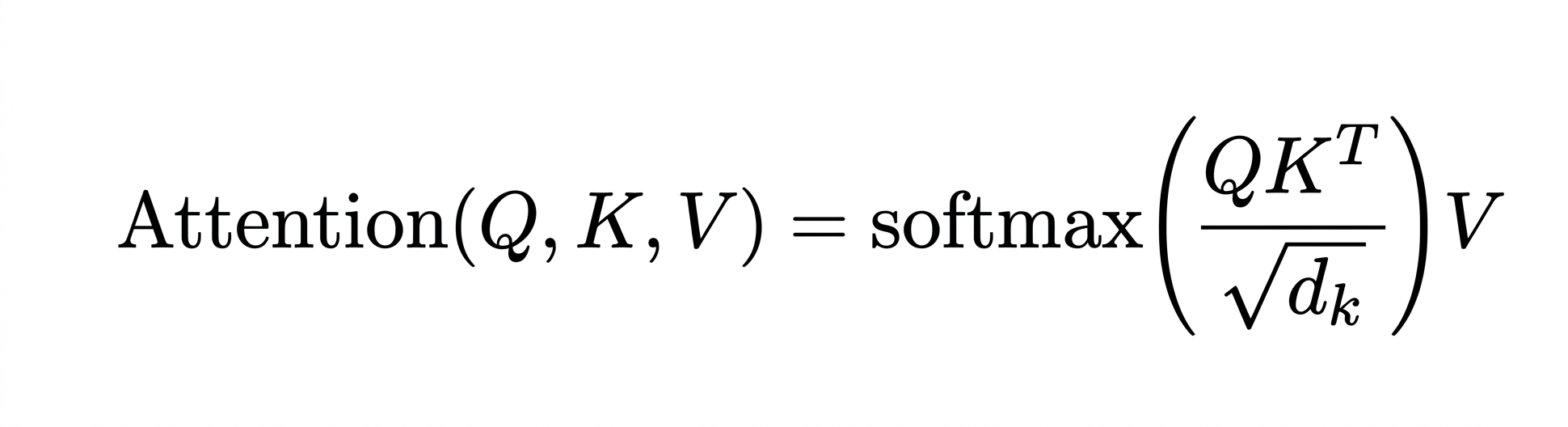
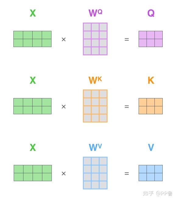
and this is how you calculate the Q, K, V matrices from said equation:
I'm tempted to, once again, outsource all the work for explaining the attention mechanism to this 3Blue1Brown video. Well, what can I say, please watch it again, it's a great video.
Without our KV Cache, the input "X" isn't just our single current token x_current, but rather it's the entire sequence thus far, [x_0, x_1, x_2, ..., x_current], where each token produces a row k_0, k_1, k_2, and so on in the final K matrix. So we have
K = X_all @ W_K    # all tokens, including x_current
V = X_all @ W_V    # all tokens, including x_current
and once we produce x_next and append that to X_all, we have the privilege of slugging through through these matrix multiplications again, yes, all of [x_0, x_1, x_2, ..., x_current, x_next]!
Remember that tiny-decode is an inference engine, and since we're doing inference, our LLM's weight matrices W_Q, W_K, and W_V don't change. They were learned during training, and now they're frozen the way they were when we finished training the LLM.
So think about what happens as our LLM reads the memo token by token. For any given token x, its K and V are just x multiplied by some fixed weight matrix. Since the weight matrices don't change, K and V for that token x will always be the same, no matter how many times the model rereads the memo.
Stop and Think
If you're wondering whether this mean that the KV cache wouldn't work during training, you'd be right. During training, we're constantly updating the weight matrices as the model learns. That means that a K and V for the same token would be different after every training step, so they cannot be stably cached. So, the KV cache is wholly an inference-time trick.
If K and V for each token never change, why recompute them every time? Just compute them once, stash them, and look them up on every subsequent pass.
q_current = x_current * W_Q

# compute the rows once
k_current = x_current * W_K
v_current = x_current * W_V
# stash the new rows in the big matrices
K = concat(K_cached, k_current) # append to cache
V = concat(V_cached, v_current) # append to cache
# look them up on each subsequent pass
scores = q_current @ K^T        # new token's Q asks for K
weights = softmax(scores / sqrt(d_k))
output = weights @ V       # and now we ask for V
So, past_key_values was holding the K and V rows for every token the model has already seen, at every layer.
Stop and Think
So why don't we cache Q too?
Caching is only useful if the same question gets asked many, many times. So what questions are we answering here, and how often do they get asked?
For K and V, the question is, "Given our currently generated token x_current, give me all of the tokens that came before it, what are their Ks and Vs?" So, for a single token x_current, that question gets asked a lot. After we generate x_current, every subsequently generated token that arrives will walk through all the tokens before it, including x_current, and ask that exact same question, "what's your K and V?" So, caching the answer pays off handsomely, since every following token in the sequence will ask about x.
Stop and Think (Within a Stop and Think)
Now, recall that we're working with a decoder. Would the KV Cache's benefits still hold for an encoder?
Recall that one difference between a decoder and an encoder is that in a decoder, every token attends to the tokens that came before it, never the ones after. Meanwhile, an encoder's where attention is bidirectional and every token attends to every other token.
In an encoder, is there still a sequential "past" to cache? Can we create one?
Meanwhile, for Q, the question would be: "Given our currently generated token x_current, what is its Q?" But who would ask that question again? Only token x itself uses its own Q, in the one moment it arrives and attends to everything before it. No future token ever needs token x's Q. So caching it would be saving an answer that isn't asked for again, which doesn't do much harm but also doesn't do much.
So, that's basically it with the KV Cache. It works because the decoder's attention only looks backward, every token's K and V are computed once and asked about forever ever after.
Phase 1, Step 5: We're Not Writing a KV Cache (Yet)
I think now's a good place to stop. Rewriting HuggingFace's DynamicCache right now would be a lot of lines of code that teach you very little you don't already understand. The gist of a KV cache is really that we had quadratic pain, and we cured it by computing each token's K and V exactly once and reusing them. The rest is implementation detail.
Instead, I want you to leave you here with a question: what happens when there's more than one person sending requests to our LLM?
Right now, we're serving a single prompt, from a single user, in one lonely decode loop. But real inference engines handle many sequences at once, and that changes a lot of things.
Suddenly, we worry for our tidy little KV Cache. The one that grows by one row each step, oh, that scrappy little grow-one-row-at-a-time cache, how will it survive the influx of user requests? How do you allocate memory for a cache when you don't know how long each sequence will be? What happens when one sequence finishes early and leaves a hole in the cache, a hole too small to use, yet too large to ignore?
In Part 2 (and maybe 3, depending on how long things get), we'll batch multiple sequences together, see how far our faithful little KV cache can carry us, and rewrite it (for real) with PagedAttention.